
Summary
•
Reverse-complement parameter sharing (RCPS)는 이론적으로 적어도 conjoined model만큼의 expressive power를 가지지만, 아마도 optimization이 어려워서 성능이 좋아지지 않는 것으로 보인다.
Abstract
•
Double-stranded DNA sequence feature를 이용해서 예측을 수행하는 모델의 경우, 이론적으로 forward strand와 reverse strand 각각을 input으로 주었을 때 동일한 예측 값을 출력해야 한다. (Reverse-complement equivariance) 그러나 대부분의 standard neural network는 그렇지 않다.
•
모델이 reverse-complement equivariance를 갖도록 하는 전략에는 두가지가 제시되어 왔지만, 어떤 전략이 더 좋은지 benchmarking이 수행되지 않아 왔다.
◦
conjoined/”siamese” architecture
◦
RC parameter sharing (RCPS)
•
본 논문에서는 base-resolution signal prediction 문제에 대해서 “post-hoc conjoined” model, 즉 개별 strand에 대해서 각각 학습을 진행한 뒤 예측 값을 aggregate하는 방식의 모델이 잘 작동함을 보이고 이를 strong baseline으로 제시한다.
•
이 post-hoc conjoining 모델은 RCPS 보다 대부분 좋은 성능을 보였고, training 과정에서 conjoining을 진행하는 “conjoined-during-training” 모델보다는 항상 성능이 좋았다.
→ RC equivariance를 달성하는 모델을 구축하기 위해서, post-hoc conjoined 모델을 reliable baseline으로 사용하고, 그것보다 성능이 좋은 모델을 구축하는 것을 목표로 하는 게 바람직하다.
Introduction
•
DNA sequence 상에 존재하는 regulatory motif를 잡아내는 데 convolutional neural network (CNN)이 널리 활용되고 있지만, Standard CNN들은 주로 computer vision task를 위해 개발되고 발전되어 왔기 때문에 double-strand DNA의 complementary base-pairing 정보를 고려하지 않는다.
◦
예를 들어 5’-GATA-3’에 binding하는 TF가 있을 때, reverse strand에 나타난 3’-CTAT-5’ signal을 보고도 forward strand에 5’-GATA-3’ 가 있다는 정보를 모델이 알아낼 수 있어야 하는데, 그게 자연스럽게 되지 않는다는 것.
◦
따라서 foward sequence를 input으로 주었을 때와, 그것의 RC version을 input으로 주었을 때의 출력 값이 매우 달라지는 경우가 많다.
◦
심지어 reverse-complement version의 sequence를 training data에 추가하여 augmentation한 경우에도 그렇다. 따라서 모델의 신뢰도가 떨어지게 되는 것.
•
초창기 Deep learning for genomics 연구들을 보면 이 문제를 forward/reverse sequence 예측을 둘다 활용함으로써 해결한다. 이런 구조를 conjoined 혹은 “siamese” architecture라고 부른다.
◦
DeepBind는 두 strand 예측 값 중 더 큰 값을 사용한다.
◦
FactorNet은 두 strand 예측 값의 평균을 사용한다.
•
결국 conjoined model은 forward/reverse strand input에 대한 “Representation merging”을 수행한다고 볼 수 있다.
•
전통적으로 representation merging을 training / testing time 둘 다 수행할 때 conjoined model 이라고 부르지만, training 시에는 representation merging을 하지 않아도 test-time에 merging을 수행하는 경우도 conjoined architecture로 볼 수 있다.
◦
Test-time에만 merging을 수행하는 이 경우, single-strand model을 post-hoc하게 conjoined model로 변환하는 것으로 볼 수 있다. (post-hoc conjoining)
•
Conjoined architecture의 단점. Conjoined architecture는 convolutional filter에 의한 motif scanning 보다 뒷 단계에서 RC equivariant가 부여되기 때문에, filter 자체는 forward motif / reverse motif 두 개가 각각 학습되어야 한다는 부담이 있다. 따라서 어떤 sequence에 어떤 motif는 forward orientation으로 있고, 어떤 motif는 reverse orientation으로 있다면 어느 한 orientation의 motif만 학습한 모델은 모든 motif를 identify할 수 없다.
→ Reverse-complement parameter sharing (RCPS)의 필요성
•
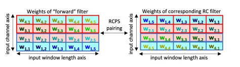
RCPS. RCPS는 window length + channel axis를 따라 flipped된 한 쌍의 weight-tied filter를 가지고 학습을 진행한다.
•
RCPS 아이디어를 사용한 연구들.
◦
Brown and Lunter : RCPS를 확장하고, dropout을 걸어 recombination hotspot detection에 활용.
◦
Bartoszewicz et al. : Pathogenic potential of novel DNA
◦
Onimaru et al. : RCPS-like concept을 가지는 layer를 고안. Forward and Reverse Sequence Scan (FRSS)라고 이름 붙임.
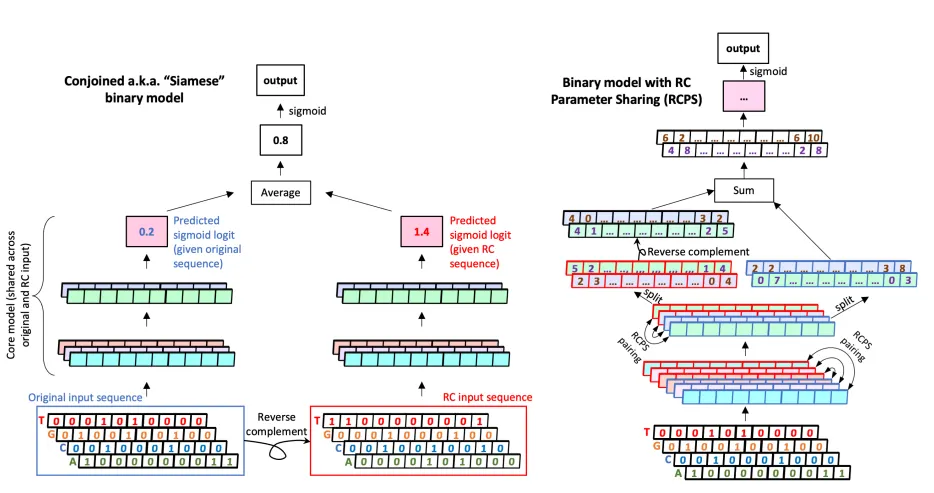
Figure 1. Conjoining과 Reverse-complement parameter sharing. (왼쪽) Conjoining의 경우 parameter가 공유되는 (Siamese) 두 개의 모델이 하나는 original sequence를 input으로 받고, 다하는 reverse-complement sequence를 input으로 받아서 두 개의 logit 값을 출력함. 두 logit을 평균내어 최종 output으로 사용. (오른쪽) RCPS의 경우 input은 original sequence만을 input으로 사용함. 다만 항상 weight가 tied된 한 쌍의 convolutional filter를 maintain하여 reverse-complement equivariance를 부여함. 즉, 이 한 쌍의 convolutional filter는 각각 forward, reverse를 담당하는 filter로서 weight 자체가 reverse-complement 관계에 있도록 학습됨.
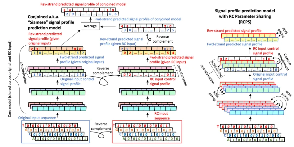
Figure 3.
Methods
Dataset
•
(1) 2개의 simulated synthetic DNA sequence dataset (200bp, 1kbp), contains motif instances sampled from 3 different TF motif models (PWM의 형태)
•
(2) Genomewise binarized TF-ChIP-seq data for MAX, CTCF, SPI1 in GM12878 lymphoblastoid cell line.
◦
Positive set : TF ChIP-seq peak 중심으로 1kbp sequence
◦
Negative set : TF ChIP-seq peak과는 겹치지 않는 DNase-seq peak 중심으로 1kbp sequence.
•
(3, basepair-level signal profile prediction) Genomewide ChIP-nexus profiles of 4 TFs (Oct4, Sox2, Nanog, Klf4) in mESC.
Model
•
(for data 1) Multi-task CNN. 주어진 sequence가 특정 motif를 가지고 있는지 판단하는 binary task를 수행함.
•
(for data 2) Single-task CNN.
•
(for data 3) BPNet-style model. TF 별로 개별 모델 학습. Multinomial loss to predict distribution of reads in 1kbp regions for each of the two strands within ChIP-nexus peaks.
Metrics
•
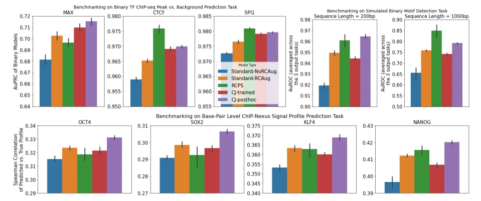
3번 데이터셋 (basepair-level signal profile prediction)을 위한 metric으로 3가지 사용 (Spearman correlation, Pearson correlation and Jensen-Shannon divergence)
◦
Profile을 probability distribution으로 볼 수 있으니 JSD를 쓸 수 있음. Predicted and true probability distributions are smoothed using a Gaussian kernel with . 개별 example과 strand 별로 측정하여 평균 값을 보고함.
◦
Correlation의 경우 1bp, 5bp, 10bp binning해서 개별 example, strand, binning resolution에 따라서 각각 correlation을 측정함. 개별 example, strand, binning resolution의 평균 값을 보고함.
Results
Post-hoc conjoined model의 성능이 trained conjoined model보다 좋다.
•
Post-hoc conjoined model
out = model(x)
out_rc = model(x_rc)
loss = criterion(out, target)
loss_rc = criterion(out_rc, target)
loss_merged = (loss + loss_rc) / 2
loss_merged.backward()
Python
복사
•
Trained conjoined model
out = model(x)
out_rc = model(x_rc)
loss = criterion((out + out_rc) / 2, target)
loss.backward()
Python
복사
•
왜 Post-hoc이 더 좋은가?
◦
(가설1) Post-hoc은 forward와 backward sequence를 이용한 예측값 둘 다 정확해져야 하지만, trained는 forward와 backward 각각은 정확하지 않아도 둘의 평균 값이 target 값과 비슷해져버리면 loss가 크게 전파되지 않는다. 따라서 더이상 학습이 진행되지 않음.
◦
(가설2) Conflicting gradients 때문에…?